Import/Catalogue/NMD 2018 Import Plan
NV NMD2018 is an import of a group of datasets which are generated from raster land use data covering (the whole area of Sweden).
The import is currently (2019-08-01) stopped. See the postmortem post describing outcomes of the project here.
A mailing list discussion for the import: March 2019 April 2019 May 2019 June 2019.
The source key value used to mark data related to this import: "NV NMD2018" in addition to "import=yes".
Goals
To increase coverage of mostly natural and land use areas in Sweden. The primary type of information expected to be imported are of types forest and meadow/grass with occasional wetlands etc.
Data coming in the raster file is documented in this PDF that came accompanying the data (in Swedish): File:NMD Produktbeskrivning NMD2018Basskikt v1 0.pdf. The forest data is a result of an AI-analysis of multi-spectral data with 13 bands in the visible, near infrared, and short wave infrared part of the spectrum from the Sentinel-2 mission.
The original GeoTIFF uses SWEREF99 (EPSG:3006) as coordinate system. Resolution of the source GeoTIFF is 10×10 meters. It covers area of the whole Sweden. Every pixel encodes type of area use, including forests and their types (coniferous, needleleaved, broadleaved, mixed etc.) roads, residential and industrial areas, lakes, rivers etc.
Schedule
- March 2019 — the raster data was made available for general public and is noted by the OSM community.
- April 2019 — technical assessment, vectorization, filtering etc. of data. Defining the strategy of import, writing plans etc, getting approvals etc.
- From end of Q2 2019 till end of 2019 — established process of submitting batches of imported data to be uploaded to the main OSM database.
- Q1-Q2 2020 — evaluate the process and solve any remaining conflation conflicts.
Import Data
Background
- Data source site: link
- Data license: CC0
- Type of license (if applicable): Public Domain with Attribution
- Link to permission (if required): at the data source page: Naturvårdsverket tillämpar licens enligt CC0. Uppge gärna källa (Källa: Nationella marktäckedata, Naturvårdsverket).
- OSM attribution: https://wiki.openstreetmap.org/wiki/Contributors#Naturv.C3.A5rdsverket
- ODbL Compliance verified: yes
OSM Data Files
Examples datasets to be uploaded. These pieces were converted manually for relatively small isolated islands with no or poor pre-existing land use coverage data.
- https://atakua.org/p/nmd/granso-fixade-fel.osm
- https://atakua.org/p/nmd/vinon-3.osm.gz
- Links to OSM files for larger areas actually planned to be uploaded can be found below and in the subpages to this page.
Import Type
This is a one time import for the year 2018 data. Data is prepared with automated scripts, then loaded into JOSM, validated with existing tools, visually controlled to be consistent and non-conflicting. It is then uploaded through JOSM interface.
If, in the future, updates for the source raster data becomes available, a different approach to import will be used. Namely, first a delta (difference) for old and new raster data will be calculated, and only those areas with significant changes in land use information will be considered for further processing.
Data Preparation
Data Reduction & Simplification
The source raster and intermediate vector data undergo the following steps:
- Import of raster data and remapping some of pixel values that would correspond to identical tags in the end.
- Existing vector OSM-data export for the country is used to create a raster mask image with coordinate system and resolution identical to those of the source file. The mask layer included zero pixel values for areas where already mapped land cover data exists. gdal_rasterize is used for this conversion.
- All input raster files (both data and mask) are split into smaller non-intersecting tiles (see reasoning behind that below).
- The raster data undergoes clean up and vectorization with gdal_vectorize. Both import data file and the raster mask file are used simultaneously under vectorization to prevent creation of polygons in the areas that are already mapped. This is important to simplify further vector data merging.
- The vector layer undergoes smoothing process: artifacts of rasterization are removed with v.generalize filter of the GRASS GIS toolset to make it look more natural. Filters used: Chaiken (threshold 20 meters) and Douglas-Peucker (threshold 0.00005 degrees or less). The first filter efficiently removes the "steps" in data, and the second one removes extraneous nodes from the dataset
- Filtering out of irrelevant data: water, residential areas, roads etc. Vector data for forests, farmland and meadows/grass are preserved.
- Scripted removal of certain types of self-intersections, duplicate nodes and duplicate polygons.
- The import data is merged with existing data in JOSM, and all boundary effects and remaining warnings caused by the import data are manually solved.
Custom scripts for raster and vector data processing related to this import are available here: https://github.com/grigory-rechistov/nmd-osm-tools. See description of these scripts in the README file of the repository.
Tagging Plans
Mapping of pixel values of original raster data to OSM tags used is described with the following Python dictionary with keys from source raster values (documented on pages 52-54) here: http://gpt.vic-metria.nu/data/land/NMD/NMD_Produktbeskrivning_NMD2018Basskikt_v1_0.pdf, mirror: File:NMD Produktbeskrivning NMD2018Basskikt v1 0.pdf)
Ignored types of the source data land cover are commented out.
Additional preliminary simplification of raster data is performed to actually merge source pixel values that have identical tags to minimize amount of polygons. E.g. pixels with values 111 and 112 are replaced with 113 etc.
Mapping of raster values to OSM tags
Note that common key/value pairs "import=yes" and "source= NV NMD2018" are added automatically to all new objects. Commented sections denote values dropped from the input raster data.
EDIT August 2019: it was additionally decided to include areas marked as wetland and water into the import process. The reasoning behind it is that many smaller and rather huge wetland areas and many small lakes are not mapped yet and would benefit from the import. As already mapped wetlands/lakes are not included into the mask layer, new overlapping conflicts may start happening. Conflation scripts have been adjusted to detect such conflicts and automatically tag and/or exclude conflicting would-be new wetland/water features from import tiles.
This Python dictionary can be found in common.py file of the Github repository for import scripts.
    # Commented are types of landuse not deemed beneficial to trace
    # 1. Water - there are better methods to trace it, also it is already traced
    #    well.
    # 2. For buildings, 10 meters resolution is not enough.
    #    NOTE maybe put a single node "building = yes" in the middle of smaller
    #    (4-8 close nodes) ways?
    # 3. Industrial - easier to trace by hand, relatively few places which are
    #    large

    ## 111 Tallskog utanför våtmark
    ## 112 Granskog utanför våtmark
    ## 113 Barrblandskog utanför våtmark
    mapper["111"]={"landuse": "forest", "leaf_type": "needleleaved", "genus": "pinus", "leaf_cycle": "evergreen"}
    mapper["112"]={"landuse": "forest", "leaf_type": "needleleaved", "genus": "picea", "leaf_cycle": "evergreen"}
    mapper["113"]={"landuse": "forest", "leaf_type": "needleleaved", "leaf_cycle": "evergreen"}

    ## 114 Lövblandad barrskog utanför våtmark
    mapper['114']={"landuse": "forest", "leaf_type": "mixed", "leaf_cycle": "mixed"}

    ## 115 Triviallövskog utanför våtmark
    ## 116 Ädellövskog utanför våtmark
    ## 117 Triviallövskog med ädellövinslag utanför våtmark
    mapper['115']={"landuse": "forest", "leaf_type": "broadleaved", "leaf_cycle": "deciduous"}
    mapper['116']={"landuse": "forest", "leaf_type": "broadleaved", "leaf_cycle": "deciduous"}
    mapper['117']={"landuse": "forest", "leaf_type": "broadleaved", "leaf_cycle": "deciduous"}

    ## 118 Temporärt ej skog utanför våtmark
    mapper['118']={"landuse": "forest", "natural": "scrub"}

    ## 121 Tallskog på våtmark
    ## 122 Granskog på våtmark
    ## 123 Barrblandskog på våtmark
    mapper['121']={"natural": "wetland", "landuse": "forest", "leaf_type": "needleleaved", "genus": "pinus", "leaf_cycle": "evergreen"}
    mapper['122']={"natural": "wetland", "landuse": "forest", "leaf_type": "needleleaved", "genus": "picea", "leaf_cycle": "evergreen"}
    mapper['123']={"natural": "wetland", "landuse": "forest", "leaf_type": "needleleaved", "leaf_cycle": "evergreen"}

    ## 124 Lövblandad barrskog på våtmark
    mapper['124']={"natural": "wetland", "landuse": "forest", "leaf_type": "mixed", "leaf_cycle": "mixed"}

    ## 125 Triviallövskog på våtmark
    ## 126 Ädellövskog på våtmark
    ## 127 Triviallövskog med ädellövinslag på våtmark
    mapper['125']={"natural": "wetland", "landuse": "forest", "leaf_type": "broadleaved", "leaf_cycle": "deciduous"}
    mapper['126']={"natural": "wetland", "landuse": "forest", "leaf_type": "broadleaved", "leaf_cycle": "deciduous"}
    mapper['127']={"natural": "wetland", "landuse": "forest", "leaf_type": "broadleaved", "leaf_cycle": "deciduous"}

    ## 128 Temporärt ej skog på våtmark
    #mapper['128']={"landuse": "forest", "natural": wetland'

    ## 2 Våtmark

    # NOTE: wetland is enabled in August 2019
    mapper['2']={"natural": "wetland"}
    ## 3 Åkermark
    mapper['3']={"landuse": "farmland"}

    ## 41 Övrig öppen mark utan vegetation
    ## 42 Övrig öppen mark med vegetation
    mapper['42']={"landuse": "grass"}

    ## 51 Exploaterad mark, byggnad
    #mapper['51']={"building": "yes", "note": "Needs surveying"}
    ## 52 Exploaterad mark, ej byggnad eller väg/järnväg
    #mapper['52']={"landuse": "industrial", "note": "Needs surveying"}
    ## 53 Exploaterad mark, väg/järnväg

    ## 61 Sjö och vattendrag
    # NOTE: water is enabled in August 2019
    mapper['61']={"natural": "water"}
    ## 62 Hav
    #mapper['62']={"natural": "water"}
The most problematic class of objects to tag turned out to be "grass". The same original raster pixel value may correspond to different concepts in OSM, ranging from a golf course, through cultivated grass to grassland and even heathland. Because of that, manual inspection of all areas tagged as "grass" is needed.
Raster masking approach
It proved difficult to automatically or even manually make sure that land use (multi)polygons from existing OSM-data and new data to be imported do not conflict with each other when they both are represented as vector outlines. Even more complex question is how to decide what to do with two conflicting ways. Should one delete one of them? Replace one with another? Merge them? Create a common border between them?
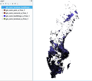
A simpler approach was developed to address conflicts at the stage when import data can be easily masked, i.e. when it is represented by raster pixels. The idea behind this approach that we can generate a second raster image of identical size and resolution for the country. The source for this raster mask image is existing OSM land cover information. For example, a vector way for already mapped forest will be turned into a group of non-zero pixels. The vectorizing software then uses this mask to prevent new vector ways to be created from the import data raster. It would look as if no data for those areas is available. As a result, vectors generated from masked raster never enter "forbidden" areas where previously mapped OSM-data is known to be present.
The picture on the right gives an overview of what areas will be covered with new data, and which will be avoided and will contain little on no new vectors. The white pixels correspond to input import data pixels that will be taken into account. All non-white pixels would look like undefined to the vectorizing software.
By restricting new data to be created only for not yet mapped areas we reduce the problem of solving polygons intersections to the problem of aligning borders between new and old polygons.
Changeset Tags
Changesets will be tagged with source = "Nationella marktackedata, Naturvardsverket" and possibly landsat imagery used as layer.
Data Transformation
Tools used:
- QGIS, GRASS, GDAL — to import raster and vector, transform and smooth vectors, visualize intermediate and final data for error checking.
- Scripts and tools (link) to convert, split, clean up, conflate data and resolve issues at intermediate steps.
- osmconvert to split a single country-wide OSM file to individual counties; [ogr2poly] to convert shapes to POLY format.
- JOSM editor to manually fix remaining issues, manually conflate with existing map features, visually and semi-automatically review changesets, and upload them to the database.
Data processing diagram
The complete data flow is illustrated on the following diagram.
    +----------------------+       +-----------------------------+
    |                      |       |                             |
    | NMD-raster image     |       | Geofabrik export data in SHP|
    |                      |       |                             |
    +------------------+---+       +--------+--------------------+
                       |                    |
                       |                    |
                       |                    | gdal_rasterize
                       |                    |
                       |           +--------v-------------------+
                       |           |                            |
                       |           | OSM raster tile in TIFF    |
                       |           |                            |
                       |           +--------+-------------------+
                       |                    |
                       |                    | negate_raster.py
                       |                    |
                       |           +--------v--------------------+
                       |           |                             |
                       |           | Mask tile (empty/not empty) |
                       |           |                             |
                       |           +-+---------------------------+
                       |             |
                       v             v
                     gdal_vectorize -mask
                              +
                              |
                              |
                    +---------v------------+
                    |                      |
                    | Vector data in GML   |
                    |                      |
                    +---------+------------+
                              |
                              | nmd-gml-to-osm.py
                              |
                    +---------v------------+        +-------------------------------+
                    |                      |        |                               |
                    | Vector data in OSM   |        | JOSM loaded actual data layer |
                    |                      |        |                               |
                    +---------+------------+        +------------------+------------+
                              |                                        |
                              +-----> Open in JOSM, merge layers, <----+
                                      fix warnings and problems
                                                +
                                                v
                                        +-------+----+
                                        |            |
                                        | Changeset  |
                                        |            |
                                        +------------+
As data spends some time inside the GRASS GIS database, the diagram below expands on what GRASS tools and external are used in order to obtain the final vector OSM-file.
           sverige.tif         sverige-mask.tif
                +                     |
                |                     |
                v                     v
    make-kommun-tiles.py       make-kommun-tiles.py
               |                      +
               |                      |
               v                      v
          tiles.tif               tile|mask.tif
                +                     |
                +----------+     +----+
                           v     v
                    gdal-polygonize.py

                    v.in.org

         v.generalize filter=chaiken threshold =20
         v.generalize filter=douglas threshold=0.00005

                    v.out.ogr

                    nmd-gml-to-osm.py
                    plow-roads.py
                    filter-osm threshold = 12
                        +
                        |
                        v
                    load into JOSM
                        +
                        |
                        v
                    fix warnings
                        +
                        v                   existing OSM data layer
                   merge layers <-------------+
                        +
                        |
                        |
                        v
                    fix warnings after merge
                        +
                        |
                        |
                        v
                      upload
Data Transformation Results
Archives for certain intermediate steps in data processing are created for inspection, backup and sharing purposes.
- Raster GeoTIFF for Sweden with small specks removed and forest types unified (projection WGS84): https://drive.google.com/open?id=1MGAJL2YLU1RXt4L8iJCg7cX2HGRrelOQ (650 MByte)
- Mask for the whole country (projection WGS84):https://drive.google.com/open?id=1Rpx-ya0dC4WSGl5JXwd0L6Ua9AhS9VPu (76 MByte) Note that pixels with value zero mean that no new vector line will be passing through that pixel in the resulting vectors.
- The mask includes rasterized data from (buffered) roads, buildings, landuse (without military and nature_reserve objects) shape layers.
- Boundaries for counties were generated by https://wambachers-osm.website/boundaries/, the request was:
wget -O boundaries.shp.zip 'https://wambachers-osm.website/boundaries/exportBoundaries?cliVersion=1.0&cliKey=individual-key&exportFormat=shp&exportLayout=levels&exportAreas=land&union=false&selected=52822&to_AL=7'. The result is available here: https://atakua.org/p/nmd/kommuner-shp.tar.bz2 (read the readme of the service to understand how to make requests to it). Note that for some reason the Gotland island was included twice as two counties, 0106 and 0218, but as it is already well mapped, no import data will be used for it. - POLY files used to extract individual counties: https://drive.google.com/open?id=1rRBdEtWY8I6AkI7sCHzpbW0zdkGCPzvd (Note: when generating POLY files, specifying boundary simplification flags to ogr2poly is very recommended)
- GeoTIFF files for counties with unified forests and WGS84 projection: https://drive.google.com/open?id=1w5vHtv_9_BVSCqeW_5C0aEAO18ZemxCM
- Resulting OSM files after conflation clean-up: see Import/NMD2018 Import status per subarea.
Older files
The files below may or may not be used under this import as they were obtained at earlier attempts to process the data.
- A raster GeoTIFF of the whole country with cleaned up areas (objects up to 4×4 pixels are removed) and unified source tag values: https://drive.google.com/file/d/12CAm3FGcjqZFgxJ5IMBdoz2yDu8MiQgY/view?usp=sharing (1.2 GB)
- Mask file for the whole country: https://drive.google.com/open?id=1uZDtIYZPOUFRPDSBTPb-jw2gk73RuwlO .
- Separate raster GeoTIFF files for individual counties (types of forest are not unified?): https://drive.google.com/open?id=1JfAidyqIdelsRj1tjrpG-OR6IkJuHxWE (WGS84)
- Separate GML vector files for counties before smoothing of "stairs" has been done: https://drive.google.com/open?id=1aVqgPf18rlEwuoAzAWHo5EgvPb5CNAb3 (4 GB)
- Filtered GML vector files with all ways shorter than 16 nodes removed: https://drive.google.com/open?id=1wOhsUxeANASwJm9h5S6FqRxX8xvHD4RF (2 GB)
- Filtered GML vector files with all ways shorter than 24 nodes removed: https://drive.google.com/open?id=12yrGmr0tfk8ohBA6vfwELqFDJD70Abhe (2 GB)
- GML files with generalized filters applied: https://drive.google.com/open?id=18eONLW6e1EoVGpwT5kTVoULggNK6Ptr3
Data Merge Workflow
Team Approach
A team of contributors collaborating through the mailing list talk-se will import data covering different parts of the country. Every contributor should create a separate account dedicated for import uploads. An intermediate unit for data import is chosen to be a county (Swedish: kommun) which are 291. Individual counties are split into rectangular tiles of identical sizes (ranging from 5×5 km to 10×10 km, currently 0.1×0.1 degrees). Tiles constitute a basic unit for this import.
The collaboration is guided through online spreadsheets or other convenient mechanisms to make sure that no two people attempt to upload the same tile twice.
Instruction for individual uploaders on how to open data files, merge with existing data and solve conflicts and warnings/errors can be found here.
References
Data will be checked using the following sources:
- Available satellite imagery, such as Maxar (ex. Digital Globe) Premium, Bing Satellite view, Mapbox Satellite View, or other sources available in JOSM.
- Existing OSM data with tags landuse, natural and other ways that will be adjacent to newly imported polygons.
- Guidelines found in this import plan and its child wiki-pages.
Workflow
- Step by step instructions:
- For the data transformation workflow steps above at "Data reduction and simplification".
- There is no need to convert the whole country from raster to vector at once. After enough data for individual counties is generated, and we got the permission to proceed, we can start uploading them.
- To distribute the workload, an assignment table "county/subarea/tile" → team member" is created (see the link below).
- The table will be used to track the progress and prevent multiple people from modifying/uploading same counties simultaneously.
- Individuals will put their names next to subareas they wish to upload. After an upload is done, it should be marked as "uploaded" in the table, with a short feedback on how well/easy it went. After its quality is rechecked, the subarea gets marked as "done".
- Proceed through all counties/subareas/tiles until all of them are finished (successfully or unsuccessfully).
- For subareas for which data upload have turned out to be problematic due to any unforeseen reasons, mark them as "failed: <reason>". A separate project will be initiated after that to address specific problems discovered along the way.
- Changeset size policy: individual changesets of this import should follow regular OSM policies on size limits.
- Revert plans: In a case of problems,
- mark all data committed with specific changeset tags associated with this import for an affected area (see above) , and/or
- mark all data committed by a specific user account under given date range;
- edit/delete data to resolve the immediate issues;
- document reasons why reverting was necessary. Later, develop a mitigation plan to address discovered issues, fix them and re-attempt uploading.
Conflation
A detailed practical guide for those who work on importing individual tiles can be found here: Catalogue/NMD_2018_Import_Plan/Rutbearbetningsprocess (in Swedish). Below is a high-level overview of issues to deal with.
Typical issues within newly imported data
This subsection gives an overview of currently known typical "inaccuracies" and artifacts that, while not being strictly harming the map, are in most cases undesirable for one or another reason. Possible mitigations of such issues are also listed.
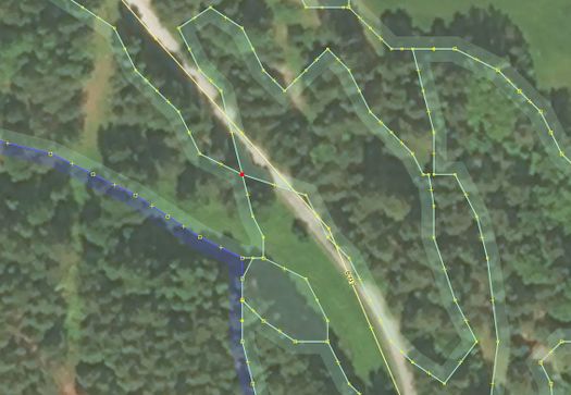
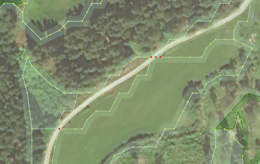
Occasional isthmuses between two land use areas separated by road
When a road goes through a forest or a field, there are often situations when a single or a small group of nodes belong to both fields, connecting them briefly. Ideally, the road should either not cross fields in such a way, or lie completely on top of a single uninterrupted field. See selected nodes on two examples below.
A manual solution can consist of:
- Delete the connecting node or node group
- Delete/fill in the empty space under the road, possibly merging land use areas it separates
An automatic solution would be to have a plugin or data processing phase that uses existing ways for roads to cut imported polygons into smaller pieces placed on different sides of that road. Then smaller ways are thrown away as artifacts. TODO write such plugin.
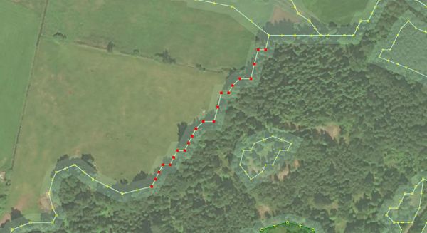
Excessively detailed ways
Often more nodes that a human would place are used on a way. Original data may have a node every 10 meters, additionally using Chaiken filter to smooth 90-degrees in vector data can create as many nodes. See an example:
A manual solution is to delete undesired nodes, and/or use "Simplify way" tool to do so.
An automatic solution would be to apply Douglas-Peucker filter to ways of the import file. The issue is to find the best threshold values for the simplification algorithm. Excessively aggressive automatic removal of nodes leads to losing important details of certain polygons. Typically it can be expected that up to 50% of import data set nodes can be removed without losing much in quality of details.
It seems that an extra pass with v.generalize douglas threshold = 0.00005 does good enough job without chewing too much of details.
Double borders between water and import land cover.
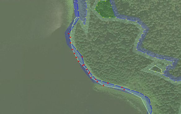
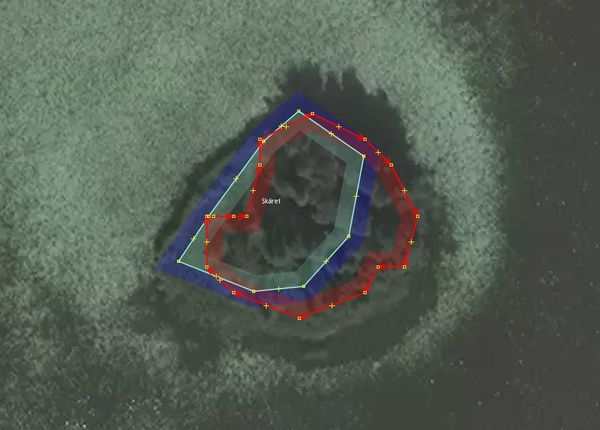
Two closely running ways of an existing shore line and a new imported forest/swamp/etc. It can also happen for already mapped islets. See two examples below.
Sometimes the previously-mapped water border is of lower quality/resolution than newly added forest bordering with it. Often both borders are equally accurate.
Manual solutions include:
- Replacing geometry for small islets.
- Deleting, merging and snapping nodes of new and old ways. ContourMerge is also useful to speed things up.
- The following plugin is created to speed up snapping of nodes of one way situated closely to another way: https://github.com/grigory-rechistov/snapnewnodes . Be sure to read the documentation and BUGS before using it.
Noisy detailed residential areas
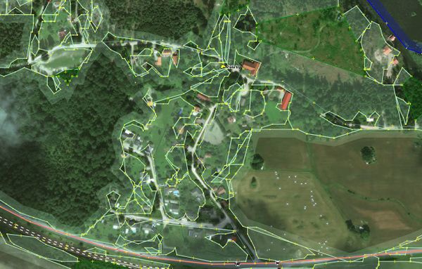
Previously unmapped areas of small farms, residential areas and similar areas with closely placed man-made features receive a lot of small polygons that are trying to fill in all empty spaces between buildings, map individual trees etc.
A manual solution is to delete all new polygons covering the area, as they are not of high value for man-made features. It is worth noticing that in most cases it is "grass" polygons with small individual areas. Selecting with a filter or search functions and then inspecting or deleting all ways tagged grass" that are smaller than a certain area could speed manual work.
No automatic solution is currently being developed or planned for the problem.
The problem does not arise with areas already mapped in OSM as they have been masked from the vectorization process and thus do not receive new polygons.
Merge strategy with existing polygons bearing "landuse", "water" or similar tags with "land cover" meaning
As import data is masked at the very first stage when it is in raster form, it is expected that areas "touching" (sharing common border) with pre-mapped land cover data will require careful examination and merging of individual way borders. All cases of overlapping of identical land uses should be fixed.
A special case is borders of water bodies and forests growing along lakes, big rivers and similar. Resolution possibilities for such cases range from leaving things as-is to using tools to merge borders into a single common one.
Interaction of new data with pre-existing linear and single-node objects
No conflicts with existing road network, power lines or similar linear objects are expected as no new linear objects are to be added. Additionally, due to specifics of the source raster data and its processing (in the source raster image there actually was data for roads as "landuse" but it is not directly used in this import), it is expected that new forest and field polygons will "wrap" around at least major roads, i.e. new polygons will not cover such roads but will stretch along them in majority of cases.
Similar reasoning applies to existing features represented as nodes. No new tagged nodes are planned to be imported. Existing nodes may become placed inside of new landuse areas, which is perfectly fine in the majority of cases.
Interaction with residential and similar areas
Areas with cities, industrial areas, water, big rivers etc. should validated with extra care during the import. If any new objects are created near or inside such areas, it should be visually controlled that new areas do not intersect with existing "landuse=residential", "landuse=industrial" etc. ways, or at least that such intersections make sense (locations with multiple landuse polygons covering them are allowed and sometimes make sense).
It should be noted that the import data tends to fill famrland's residential areas with many small polygons that are placed in between buildings. Such situations require manual clean up before uploading as there is no use of tagging every individual tree with a tiny "natural=forest" area., or similar.
Import status per sub-area
Status of imports of individual sub-areas (initially assigned to counties) is tracked here: Import/NMD2018 Import status per subarea.
Quality Assurance Plan
- At all stages when vector data is loaded into JOSM, the standard JOSM/Validator will be used to detect inconsistencies.
- It is a requirement for this import that no errors detected by the validator are uploaded together with the new data. When possible, even older errors have to be fixed along with the upload (and committed in separate changesets). No new warnings caused by the new data being imported are allowed. It is encouraged to fix pre-existing warnings for areas that are being updated right before the import changeset uploading. However, if it turns out to be too problematic to achieve, it is allowed to let previously created warnings that are not affected by newly added polygons stay.
- After individual stages of data import for specific counties are finished, the Osmose web service will be used to detect any remaining errors/warnings. To simplify detection of problems caused by this particular import, the per-user problem reporting will be used: http://osmose.openstreetmap.fr/en/byuser/ for the dedicated import account.
See also
The email to the Imports mailing list was sent on 2019-04-14 and can be found in the archives of the mailing list at https://lists.openstreetmap.org/pipermail/imports/2019-April/005958.html.
- The talk-se mailing list: https://lists.openstreetmap.org/listinfo/talk-se
- The main thread dedicated to the import process: https://lists.openstreetmap.org/pipermail/talk-se/2019-April/003547.html
- Diary entries on the conflation process: https://www.openstreetmap.org/user/Atakua/diary/
