TopOSM/Details

Data Sources

Most of the map feature data comes from OpenStreetMap. I used Cloudmade's OSM database extracts for Massachusetts.

Contour lines come from the MassGIS Elevation Contours (1:5000) data layer.

MassGIS has an 1:5000 DEM data layer. Unfortunately this layer is not available for download. The corresponding 1:5000 Shaded Relief layer is available, however, so this layer was used for the hillshading.

Additionally, since the OSM data (at time of writing) lacks many of the hydrographic features (lakes, wetlands, rivers etc), I also downloaded the MassGIS Hydrography (1:25000) data layer.

Since many of the data sources are quite large, they were imported into a PostGIS database. This process is described in many other places, such as Mapnik#osm2pgsql.

I had some initial trouble re-projecting on the fly during rendering. However, reprojecting all shapefiles to Lat-Long/WGS84 (as suggested by some other articles) seemed to solve the problems. This can be done with a tool such as ogr2ogr (part of the GDAL toolset). As an example, this is a script that transforms each shapefile in SRCDIR from SOURCE_SRS to DEST_SRC, placing the output in DESTDIR:

#!/bin/bash
# Reprojects all shapefiles in source dir to dest dir, given the
# specified source and dest spatial reference systems

SRCDIR="hydrography"
DESTDIR="hydrography-llwgs84"
SOURCE_SRS="+proj=lcc +lat_1=41.71666666667 +lat_2=42.68333333333 +lat_0=41 +lon_0=-71.5 +x_0=200000 +y_0=750000"
DEST_SRS="+proj=latlong +datum=WGS84"

for FILE in $SRCDIR/*.shp; do
    BASEFILE=`basename "$FILE"`
    echo "Reprojecting ${FILE}..."
    ogr2ogr -f "ESRI Shapefile" \
	-s_srs "$SOURCE_SRS" -t_srs "$DEST_SRS" \
	"$DESTDIR/$BASEFILE" \
	"$SRCDIR/$BASEFILE"	
done

Licensing

OSM Data is available under the Creative Commons "Attribution-Share Alike" (CC-BY-SA) license. MassGIS data is free for any use, as long as proper attribution is given. Therefore, this topo map is available under the CC-BY-SA license as well.

Process overview

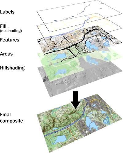
The map is rendered as 256x256 pixel tiles that can be viewed with OpenLayers, just like other OpenStreetMap layers. For each tile of the topo map, several images are generated using different methods and then finally combined into one tile.

Hillshading

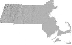
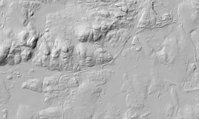
The hillshading forms the base of the final tile, onto which other map features are "pasted". The MassGIS Shaded Relief layer comes as one large (some 30k by 19k pixel) GeoTIFF image.

MassGIS shaded relief layer.

Fixing the surrounding areas

As expected in a shaded relief layer, neutral areas are middle gray, north/west facing slopes are light and south/east facing slopes are dark. Areas outside of Massachusetts in this layer are white, which would later turn out to be a problem since I didn't have a precise way to mask these areas. This became particularly problematic around the coastlines.

In the end, I loaded the image into GIMP and made them neutral gray. Unfortunately GIMP, as most image editors, does not preserve GeoTIFF tags, so I had to put these back. At the very least, I will need projection and corner coordinates to correctly split the image into tiles. The projection for MassGIS raster layers is a Lambert Conformal Conic projection, described here.

Shaded relief, after modifications.

I did not find any of the tools to copy GeoTIFF tags to work, but this can also be done using the GDAL tools. Here, shderel5k.tif is the original image and shdrel5k_cleaned.tif is the image after modifications with GIMP.

$ gdalinfo shdrel5k.tif
[...]
Corner Coordinates:
Upper Left  (   32895.000,  962105.000) ( 73d32'45.11"W, 42d53'29.52"N)
Lower Left  (   32895.000,  773895.000) ( 73d29'31.41"W, 41d11'51.22"N)
Upper Right (  333115.000,  962105.000) ( 69d52'12.58"W, 42d53'53.25"N)
Lower Right (  333115.000,  773895.000) ( 69d54'46.91"W, 41d12'14.33"N)
Center      (  183005.000,  868000.000) ( 71d42'19.21"W, 42d 3'43.97"N)
[...]

$ gdal_translate -a_ullr 32895 962105 333115 773895 -a_srs "+proj=lcc
+lat_1=41.71666666667 +lat_2=42.68333333333 +lat_0=41 +lon_0=-71.5 +x_0=200000
+y_0=750000 +datum=nad83" shdrel5k_cleaned.tif shdrel5k_cleaned_georef.tif

Cutting tiles

For each map tile, the corresponding part needs to be extracted from the Shaded Relief layer. Since the data uses a different projection than OSM (whose projection I chose to use for the final map), this process involves reprojecting the data as well. GDAL to the rescue, once again!

This script uses gdalwarp to reproject and extract a part of the image specified by its command line parameters.

#!/bin/bash

# syntax: hillshade <width> <height> <xmin> <ymin> <xmax> <ymax> <out.tif>

# default SRS for OSM
DEST_SRS="+proj=merc +a=6378137 +b=6378137 +lat_ts=0.0 +lon_0=0.0 +x_0=0.0 +y_0=0 +k=1.0 +units=m +nadgrids=@null +no_defs +over"

WIDTH=$1
HEIGHT=$2
XMIN=$3
YMIN=$4
XMAX=$5
YMAX=$6
TEMPIMAGE="`mktemp`.tif"
SRCIMAGE="/home/lars/projects/mapnik-osm/topomap/shaded-relief/shdrel5k_cleaned_georef.tif"
DESTIMAGE=$7
INTERP=lanczos
gdalwarp -q \
    -t_srs "$DEST_SRS" \
    -te $XMIN $YMIN $XMAX $YMAX \
    -ts $WIDTH $HEIGHT \
    -r $INTERP \
    "$SRCIMAGE" "$TEMPIMAGE"
convert -quiet "$TEMPIMAGE" "$DESTIMAGE"
rm "$TEMPIMAGE"

Gdalwarp offers different types of interpolation methods. For the highest zoom levels, we need every bit of resolution and quality we can get. Therefore the highest quality (but also most computationally intensive) Lanczos interpolation was chosen.

Area colors

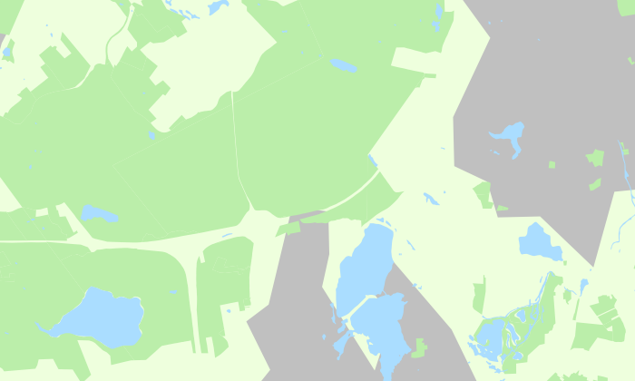
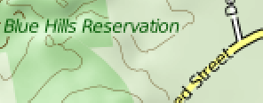
Areas such as forests and parks (green), populated areas (gray), tidal flats (gray-green) etc are rendered using Mapnik onto a separate layer which is later combined with the hillshading.

This mapnik style file is used to render areas.

Map features

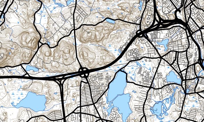
Map features, such as roads, lakes, rivers, contours and points of interest are rendered as a separate image. The reason for this is that while areas, such as forests, should be shaded with the hillshading layer, these map features should not. Thus, this image is rendered with a transparent background, and can simply be pasted on top in the final composite.

This mapnik style file is used to render features.

Labels

The "halo" effect, at 200%. Note that road fills are visible behind labels, despite the "halo".

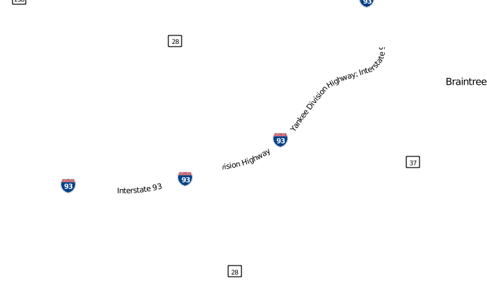
Labels and highway shields are rendered as yet another image. The reason for this is the type of "halo" used for labels. Rather than outlining text with a white halo, I prefer a gap between the text and other high-contrast features, similar to high-quality printed maps. To achive this, the map features and labels are rendered separately, and in the final composite the latter "casts" a halo while the former "receives" it.

Extracting the route numbers (for highway shields) requires some tricks when querying the database. See comments in the style file.

This mapnik style file is used to render labels.

Non-shaded areas (fill)

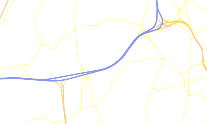
Some low-contrast features, such as road fills, are rendered on a separate layer, so that they are visible underneath labels despite the halo method mentioned above.

This mapnik style file is used to render non-shaded areas.

Combining images into a final composite

The following script takes the individual images for one tile on the command line and combines them using the ImageMagick convert program.

#!/bin/bash

# syntax: combine <area> <areansh> <features> <hillshade> <labels> <output>

AREATILE=$1
AREANSHTILE=$2
FEATURESTILE=$3
HILLSHADETILE=$4
LABELSTILE=$5
DESTIMAGE=$6

# Gamma values for hillshade highlight and shadows
# NOTE: *lower* these values for a more pronounced effect
LIGHT_GAMMA=0.8
DARK_GAMMA=1.0

# The combine-tiles-command-line-of-doom
# (though more efficient than creating loads of temp files and
# invoking IM 10 times or so per tile...)
convert "$AREATILE" \
	\( "$HILLSHADETILE" -level 70,90%,$LIGHT_GAMMA \) \
	-compose screen -composite \
	\( "$HILLSHADETILE" -level 0,80%,$DARK_GAMMA \) \
	-compose multiply -composite \
	\( \
		-size 256x256 xc:black \( "$LABELSTILE" -channel \
		Alpha -blur 0x2.0 -channel matte -separate +channel -negate \
		-level 5,8% \) -compose Copy_Opacity -composite \
		"$FEATURESTILE" -compose Src_Out -composite \
	\) -compose src_atop -composite \
	"$AREANSHTILE" -compose src_atop -composite \
	"$LABELSTILE" -compose src_atop -composite \
	"$DESTIMAGE"

Illustration of how the individual images are combined.

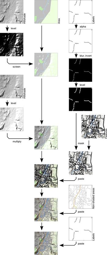
To improve performance and avoid writing lots of temporary files, the compositing is performed in one step, leading to a rather scary command line, but we can dissect it. See the chart for an illustration of what actually happens in these steps, and what is generated in the interim steps.

First, the area image is loaded.

The first internal sub-image (within parentheses) adjusts the levels in the hillshade tile so that only highlights remain - everything else is black, which is then composited onto the area image using the "screen" operator. Similarly, the shadow sections are extracted from the hillshade and composited using "multiply". The contrast of the shadows and highlights can be controlled using the gamma values in the script. Separating highlights and shadows this way gives great control over the hillshading.

The next, large, parenthesized block loads the features layer and removes the "halos" around where the labels will go. Lacking a more efficient method, this is essentially done by loading the labels, extracting the alpha channel, blurring it and applying a threshold on the result (that's what the -level 5,8% does) to create an outline. Then, that channel is treated like a mask that is applied to the features image, which is finally pasted on top.

Finally, the non-shaded areas and labels are simply pasted on top.

Batch generation

Now that the required scripts are in place, they can be driven by a modified version of the python mapnik script:

generate_topo.py

This script takes the min and max zoom levels to render on the command line. Additionally, it takes a start and end parameter, used to render sub-areas. For example, to render zoom 12 to 16 of the western quarter of the area specified in the script, call it with:

$ ./generate_topo.py 12 16 0 0.25

This start and end parameters are particularly useful when running several instances simultaneously for faster rendering on multi-core processors.

The script will skip rendering any image that already exists, so that all image types don't need to be re-rendered when making a small change to one of the mapnik style files.

The final result.

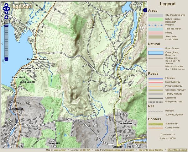
Map legend

The legend.py script is used to generate an HTML legend (with images) for a specified zoom level.

The script takes an XML description file as input, containing a list (or hierarchy) of sections and features to be included in the legend, and the tags that these features would have. This file also specifies what Mapnik XML configuration file(s) to look in.

As an example, this is the XML file describing the legend for TopOSM:

<?xml version="1.0" encoding="utf-8"?>
<legend>

	<input>../topo-area.xml</input>
	<input>../topo-features.xml</input>
	<input>../topo-areansh.xml</input>

	<title>Legend</title>

	<group>
		<title>Areas</title>
		<drawAs>area</drawAs>	
		<feature name="City, Populated area">
			<style>builtup</style>
		</feature>
		<feature name="Nature reserve, Recreation">
			<style>areas</style>
			<tag k="leisure" v="nature_reserve"/>
		</feature>
		<feature name="Wetland">
			<style>wetland</style>
			<tag k="SYM_COMM" v="WETLAND"/>
		</feature>
		<feature name="Tidal flat, Marsh">
			<style>surface-water</style>
			<tag k="sym_comm" v="FLATS"/>
		</feature>
		<feature name="Military">
			<style>areas</style>
			<tag k="landuse" v="military"/>
		</feature>
		<feature name="Area under construction">
			<style>areas</style>
			<tag k="landuse" v="construction"/>
		</feature>
	</group>
	
	<group>
		<title>Natural</title>
		<feature name="River, Stream">
			<drawAs>line</drawAs>
			<layer>line-water</layer>
			<tag k="ARC_CODE" v="4"/>
		</feature>
		<feature name="Ocean, Lake, Reservoir">
			<drawAs>area</drawAs>
			<layer>surface-water</layer>
			<tag k="sym_comm" v="SURFACE WATER"/>
		</feature>
		<feature name="Contour line">
			<remark>30 m (~98.4 ft) interval</remark>
			<style>contoursheavy</style>
			<drawAs>line</drawAs>
		</feature>
		<feature name="Minor contour line">
			<remark>3 m (~9.8 ft) interval</remark>
			<style>contours</style>
			<drawAs>line</drawAs>
		</feature>
	</group>
	
	<group>
		<title>Roads</title>
		<drawAs>line</drawAs>
		<style>roads</style>
		<feature name="Interstate">
			<tag k="highway" v="motorway"/>
		</feature>
		<feature name="Major highway">
			<tag k="highway" v="trunk"/>
		</feature>
		<feature name="Primary highway">
			<tag k="highway" v="primary"/>
		</feature>
		<feature name="Secondary highway">
			<tag k="highway" v="secondary"/>
		</feature>
		<feature name="Tertiary highway">
			<tag k="highway" v="tertiary"/>
		</feature>
		<feature name="Local road">
			<tag k="highway" v="residential"/>
		</feature>
		<feature name="Unimproved road">
			<tag k="highway" v="track"/>
		</feature>
	</group>
	
	<group>
		<title>Rail</title>
		<style>roads</style>
		<drawAs>line</drawAs>
		<feature name="Railroad">
			<tag k="railway" v="rail"/>
		</feature>
		<feature name="Subway, Light rail">
			<tag k="railway" v="light_rail"/>
		</feature>
	</group>
	
	<group>
		<title>Borders</title>
		<drawAs>line</drawAs>	
		<feature name="State border">
			<layer>state-borders</layer>
			<tag k="coast" v="N"/>
		</feature>
		<feature name="County border">
			<layer>county-borders</layer>
		</feature>
	</group>
	
</legend>

The <group> tag lets you group features visually, and lets you specify common details. You can place features directly under <legend>, or you can nest groups as deeply as you wish.

The legend and each group may have a <title>.

For each feature, you specify the name (description) that is shown on the legend. Typically you'll also specify the tags that the type of feature would have. Optionally, a feature may have a remark, that will be added to the output.

You specify whether the feature should be rendered as a line <drawAs>line</drawAs> or as an area <drawAs>area</drawAs>. You can also limit a feature or group of features to a specific layer or style in the mapnik XML file.

Note that "drawAs", "style" and "layer" are inherited, so you can specify it per group, or even directly under <legend>. You can also specify the common value in a parent element, and override it further down where necessary.

The HTML is output to stdout, and the images are placed in the specified directory (or images/ by default). Run legend.py --help for command line options.

Since the script outputs the legend for a specific zoom level, to generate all zoom levels, you can do something like:

lars@titan$ for z in {6..16}; do ./legend.py -z $z legend.xml > $z.html; done

Finally, simply style the output using CSS. This is the style from TopOSM.com:

#legend {
	position: fixed;
	top: 5px;
	bottom: 20px;
	right: 5px;
	width: 190px;
	overflow: auto;
	font-size: 70%;
}
#legend h1 { padding: 0px; margin: 0 0 10px 0; text-align: center; }
#legend h2 { padding: 0px; margin: 5px 0 5px 0; }
#legend .feature { clear: both; }
#legend .feature img { float: left; }
#legend .feature .name { margin-left: 85px; }
#legend .feature .remark { margin-left: 85px; font-size: 90%; }
#legend #zoomLevel { clear: both; text-align: center; margin-top: 20px; }
#legend #scale { clear: both; text-align: center; margin-top: 5px; }

How the script works

Internally, the script works as follows:

• It parses the legend description file into a dictionary based tree-like structure (see parseDescriptionFile).
• It processes each Mapnik configuration file in the order specified (see processMapnikConfigFile). For each such file:
  • For each referenced style in each layer (data source):
    • The script traverses the description tree (processGroup), looking for features that match the layer and style, if specified (processFeature). If there is a match, it checks each rule whether the rule applies to the current zoom level and whether the feature passes any filter criteria.
    • For every rule that passes all of these tests, each of is symbolizers is examined and drawn (if supported) using cairo. Note that many rules can match a single feature (for example, roads are typically drawn as a light stroke (fill) on top of a wider darker stoke (outline)).
• Finally the description tree is traversed again (see "export"), creating HTML and writing images do disk. Only features that were actually drawn are exported.

There are several limitations to this approach. Some of these limitations are noted at the top of the source file. The script was created specifically for TopOSM, but can probably be extended if necessary. Also, my day job is curly-brace coding - not python - so forgive me for (or fix) anything that looks odd or un-pythonic.

An alternative approach would have been to try to "fake" a Mapnik data source and let mapnik render it. This would avoid having to "emulate" Mapnik's parsing and rendering. As far as I can tell, however, there is no elegant way of doing this.